The `KEGGemUP` package: building KEGG pathway graphs and mapping real data results
Edoardo Filippi
Institute of Medical Biostatistics, Epidemiology and Informatics (IMBEI), MainzDeparment of Nephrology, Mainz University Medical Centeredoardo.filippi@uni-mainz.de
Federico Marini
Institute of Medical Biostatistics, Epidemiology and Informatics (IMBEI), Mainzfederico.marini@uni-mainz.de
23 February 2026
Source:vignettes/kegg-graph-real-data.Rmd
kegg-graph-real-data.RmdCompiled date: 2026-02-23
Last edited: 15-12-2025
License: MIT + file LICENSE
Installation
The first step is installing the package. If you dont have the package installed you can do so by running:
install.packages("remotes")
remotes::install_github("edo98811/KEGGemUP")
Then load it.
KEGG pathways are used in many bioinformatics contexts, this package package can make it very easy to implement these in the analysis of real data.
A very important part of bioinformatics analyses is both data integration and visiazionation. KEGGemUP aims to facilitate these tasks by providing functions to parse KEGG pathways and build graph objects, the idea is then to use these graph to map on them thre results of differential expression analyses.
KEGG database uses pathway ids to identify each pathway, for example “hsa00563” is the KEGG pathway ID for “Glycosylphosphatidylinositol (GPI)-anchor biosynthesis” in humans. You can use these pathway IDs to download the KGML files for each pathway and then parse them to build graph objects. The id must have the organism prefix, for example “hsa” for human pathways, “mmu” for mouse pathways, etc.
These vignette assumes you have already performed a differential
expression analysis and have the results available as a
data.frame (which you can easily obtain from edgeR or limma
by running as.data.frame() on the table of the results for
each object). To reproduce this situation we will now build an example
of a differential expression result using the macrophage dataset from
the macrophage package: bioconductor
page
To learn more about graph manipulation you can refer to the igraph and visNetwork documentation:
- igraph Is a package for creating and manipulating graphs in R.
- visNetwork Is a package for interactive visualization of graphs in R, an R interface to the javascript library vis.js.
message("--- Loading packages...")
#> --- Loading packages...
suppressPackageStartupMessages({
  library("macrophage")
  library("org.Hs.eg.db")
  library("SummarizedExperiment")
  library("AnnotationDbi")
  library("clusterProfiler")
  library("limma")
  library("igraph")
  library("edgeR")
})
message("- Done!")
#> - Done!

# Load the macrophage dataset ---------------------------------------------------
data(gse)
rownames(gse) <- substr(rownames(gse), 1, 15)  # truncate rownames at 15 characters

# limma analysis ---------------------------------------------------------------
condition <- factor(colData(gse)[, "condition_name"])
design <- model.matrix(~0 + condition)

contrast.matrix <- makeContrasts(
  IFNg_vs_naive = conditionIFNg - conditionnaive,
  levels = design
)

dge <- DGEList(assay(gse))
dge <- calcNormFactors(dge)

cutoff <- 1
drop <- which(apply(cpm(dge), 1, max) < cutoff)
dge <- dge[-drop, ]

voom_mat <- voom(dge, design, plot = FALSE)
fit <- lmFit(voom_mat, design)
fit2 <- contrasts.fit(fit, contrast.matrix)
fit2 <- eBayes(fit2)  # Empirical Bayes moderation

# Gene annotation ---------------------------------------------------------------

anns <- AnnotationDbi::select(
  org.Hs.eg.db,
  keys = rownames(gse),
  columns = c("SYMBOL", "ENTREZID"),
  keytype = "ENSEMBL",
  multiVals = "first"
)
#> 'select()' returned 1:many mapping between keys and columns

# limma results ---------------------------------------------------------------
res_macrophage_IFNg_vs_naive_limma <- topTable(
  fit2,
  coef = "IFNg_vs_naive",
  adjust = "fdr",
  number = Inf,
  confint = TRUE
)

res_macrophage_IFNg_vs_naive_limma$ENTREZID <- anns$ENTREZID[match(rownames(res_macrophage_IFNg_vs_naive_limma), anns$ENSEMBL)]

# Enrichment analysis ----------------------------------------------------------
de_entrez_IFNg_vs_naive_genes <- anns $ENTREZID[
  (!is.na(res_macrophage_IFNg_vs_naive_limma$adj.P.Val)) &
    (res_macrophage_IFNg_vs_naive_limma$adj.P.Valj <= 0.05)
]
Building KEGG pathway graphs and mapping real data results
Exporting the graph
This is how to build a KEGG pathway graph and the structure of its nodes and edges.
graph <- kegg_to_graph("hsa00563")
#> adding rname 'https://rest.kegg.jp/get/hsa00563/kgml'

# Extract all vertex attributes
vertices_df <- igraph::as_data_frame(graph, what = "vertices")

# Extract all edge attributes
edges_df <- igraph::as_data_frame(graph, what = "edges")

DT::datatable(
  vertices_df,
  options = list(scrollX = TRUE)
)Building KEGG pathway graphs
You can build a KEGG pathway graph from a KEGG pathway ID using the
function kegg_to_graph(). The input of this function is a
KEGG pathway ID (for example “hsa00563” for the human
Glycosylphosphatidylinositol (GPI)-anchor biosynthesis pathway) and the
output is a graph object representing the pathway.
Build a graph from a pathway ID and map results to nodes
To map the differential expression results to the nodes of a KEGG
pathway graph you can use map_results_to_nodes(). The input
of this function is a graph object built with
kegg_to_graph() and a list of differential expression
results tables or a single differential expression results table.
You can also pass as input to map_results_to_nodes() a
single data.frame with the differential expression results.
This dataframe must contain at least two columns: one with the KEGG
feature IDs (without organism prefix) and another with the values to map
to the nodes (e.g., log2 fold changes). You can pass to the function the
names of these columns if they differ from the default ones with the
parameters feature_column and
value_column.
Note that the KEGG IDs without organism prefix are the the ENTREZ IDs for genes. For other feature types (e.g., compounds) you will need to make sure that the IDs in your differential expression results table match the KEGG IDs used in the graph.
The defualt parameters are:
-
feature_column: “KEGG_ids” -
value_column: “log2FoldChange”
If you have multiple differential expression results tables (for example if you have one metabolomics and one transcriptomics) to map to the nodes you can pass a list of lists. Each sublist must contain the following elements:
-
de_table: a data.frame with the differential expression results. -
value_column: the name of the column in de_table containing the values to map to the nodes. -
feature_column: the name of the column in de_table containing the feature IDs (e.g., ENTREZ IDs) that correspond to the KEGG ids in the graph (without organism prefix).
This is an example of how to build such a list of differential expression results tables. In this case there is only one element, but ideally you would have one for each omics layer or source you want to map to the graph nodes.
de_results_list <-list(
  trans_limma = list(
    de_table = data.frame(res_macrophage_IFNg_vs_naive_limma),
    value_column = "logFC",
    feature_column = "ENTREZID"
  )
)
Example of usage with the list of DE results tables
We will now take a KEGG pathway from the enrichment results we built earlier and map the differential expression results to its nodes. As you can see you simply need to pass to the function the graph object and the list of differential expression results tables that we defined before.
The workflow is as follows: first we build the graph from the KEGG
pathway ID, then we map the differential expression results to the nodes
of the graph, and at the end we plot the graph using
make_kegg_visNetwork(), which creates an interactive
visualization of the graph using visNetwork.
pathway <- "hsa00563"
graph <- kegg_to_graph(pathway, scaling_factor = 10)
graph <- map_results_to_graph(graph, de_results_list)
#> Warning in vertices_df$de_text[ids_nodes_to_check] <-
#> format(round(as.numeric(vertices_df$de_value), : number of items to replace is
#> not a multiple of replacement length
graph_visnetwork <- make_kegg_visNetwork(graph)
graph_visnetwork
Example of usage with a single DE results table
Let’s first build a filtered differential expression results table with only the significant results.
de_results_limma <- data.frame(res_macrophage_IFNg_vs_naive_limma)Then we will call the function with this table as input. The
parameter feature_column and value_column are
set to match the column names in our differential expression results
table.
graph <- kegg_to_graph(pathway)
graph <- map_results_to_graph(graph, de_results_limma, feature_column = "ENTREZID", value_column = "logFC")
#> Using provided value_column: 'logFC'
#>  and provided feature_column: 'ENTREZID'.
#> de_results provided as a single data.frame.
#> Warning in vertices_df$de_text[ids_nodes_to_check] <-
#> format(round(as.numeric(vertices_df$de_value), : number of items to replace is
#> not a multiple of replacement length
graph_visnetwork <- make_kegg_visNetwork(graph)
graph_visnetwork
You can also control the palette that is used to map the values to
colors on the nodes with the parameter palette. The default
is “RdBu” from RColorBrewer, but you can use any palette supported by
RColorBrewer. To see the available palettes you can run
RColorBrewer::display.brewer.all(). You can also visit this
page: RColorBrewer
palettes.
graph <- kegg_to_graph(pathway)
graph <- map_results_to_graph(graph, de_results_limma, feature_column = "ENTREZID", value_column = "logFC", palette = "PiYG")
#> Using provided value_column: 'logFC'
#>  and provided feature_column: 'ENTREZID'.
#> de_results provided as a single data.frame.
#> Warning in vertices_df$de_text[ids_nodes_to_check] <-
#> format(round(as.numeric(vertices_df$de_value), : number of items to replace is
#> not a multiple of replacement length
graph_visnetwork <- make_kegg_visNetwork(graph)
graph_visnetwork
Igraph Visualisation
Let’s build another pathway as example:
library(AnnotationDbi)
library(org.Mm.eg.db)
#>

pathway <- "mmu00230"

g <- kegg_to_graph(pathway) |>
  map_results_to_graph(de_results_list)
#> adding rname 'https://rest.kegg.jp/get/mmu00230/kgml'
it can happen that you only want a subset of it, expecially for
complex pathways. For that therfe is the function
make_graph_subset. You need to supply to it either
entrezids for gene and proteins, or KEGG compound ids if you wish to use
the compounds. We can make a subset of it and try to visualise it using
the igraph function.
KEGG_to_include <- c("C00262", "C00385", "C00366", "C00294", "C00387",
                 "C01762", "C05512", "C00301", "C01185", "C00455",
                 "22436", "14544", "18950", "11486", "80285", "59027")
subg <- make_graph_subset(g, KEGG_to_include)

make_igraph_visualisation(subg)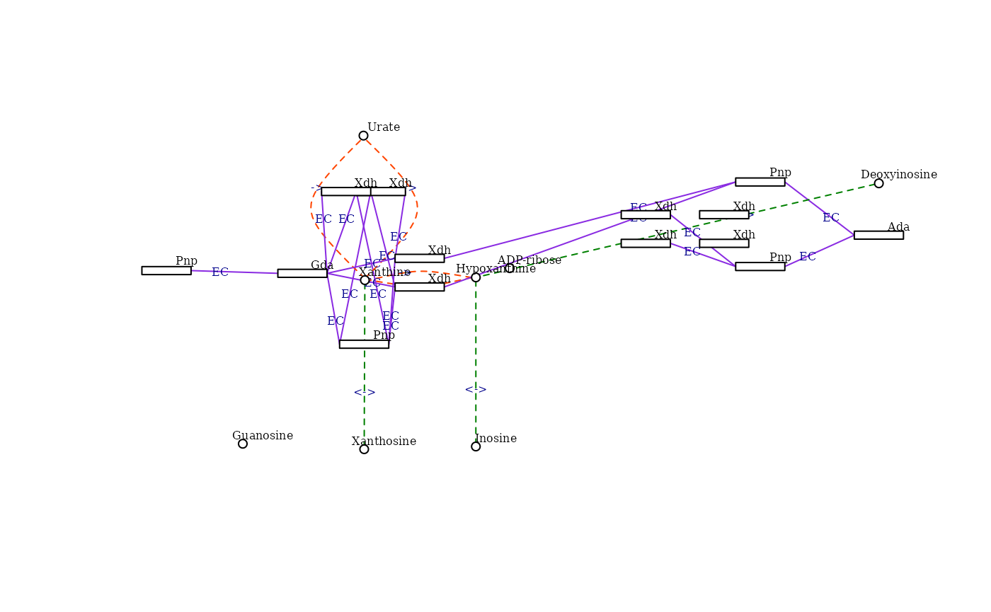
Loading a downloaded file
You can also download a kgml file from kegg and parse a kegg pathway directly from it.
path_file <- KEGGemUP::download_kgml( "mmu04933")

graph_parsed <- kegg_to_graph(pathway_id = "example", kgml_file = path_file)
#> Warning in value[[3L]](cond): Could not retrieve pathway name for ID: example

make_kegg_visNetwork(graph_parsed)
Session info
sessionInfo()
#> R version 4.5.2 (2025-10-31)
#> Platform: x86_64-pc-linux-gnu
#> Running under: Ubuntu 24.04.3 LTS
#>
#> Matrix products: default
#> BLAS:   /usr/lib/x86_64-linux-gnu/openblas-pthread/libblas.so.3
#> LAPACK: /usr/lib/x86_64-linux-gnu/openblas-pthread/libopenblasp-r0.3.26.so;  LAPACK version 3.12.0
#>
#> locale:
#>  [1] LC_CTYPE=C.UTF-8       LC_NUMERIC=C           LC_TIME=C.UTF-8
#>  [4] LC_COLLATE=C.UTF-8     LC_MONETARY=C.UTF-8    LC_MESSAGES=C.UTF-8
#>  [7] LC_PAPER=C.UTF-8       LC_NAME=C              LC_ADDRESS=C
#> [10] LC_TELEPHONE=C         LC_MEASUREMENT=C.UTF-8 LC_IDENTIFICATION=C
#>
#> time zone: UTC
#> tzcode source: system (glibc)
#>
#> attached base packages:
#> [1] stats4    stats     graphics  grDevices utils     datasets  methods
#> [8] base
#>
#> other attached packages:
#>  [1] org.Mm.eg.db_3.22.0         edgeR_4.8.2
#>  [3] igraph_2.2.2                limma_3.66.0
#>  [5] clusterProfiler_4.18.4      SummarizedExperiment_1.40.0
#>  [7] GenomicRanges_1.62.1        Seqinfo_1.0.0
#>  [9] MatrixGenerics_1.22.0       matrixStats_1.5.0
#> [11] org.Hs.eg.db_3.22.0         AnnotationDbi_1.72.0
#> [13] IRanges_2.44.0              S4Vectors_0.48.0
#> [15] Biobase_2.70.0              BiocGenerics_0.56.0
#> [17] generics_0.1.4              macrophage_1.26.0
#> [19] KEGGemUP_0.1.0
#>
#> loaded via a namespace (and not attached):
#>   [1] RColorBrewer_1.1-3      jsonlite_2.0.0          tidydr_0.0.6
#>   [4] magrittr_2.0.4          ggtangle_0.1.1          farver_2.1.2
#>   [7] rmarkdown_2.30          fs_1.6.6                ragg_1.5.0
#>  [10] vctrs_0.7.1             memoise_2.0.1           ggtree_4.0.4
#>  [13] htmltools_0.5.9         S4Arrays_1.10.1         curl_7.0.0
#>  [16] SparseArray_1.10.8      gridGraphics_0.5-1      sass_0.4.10
#>  [19] bslib_0.10.0            htmlwidgets_1.6.4       desc_1.4.3
#>  [22] plyr_1.8.9              httr2_1.2.2             cachem_1.1.0
#>  [25] lifecycle_1.0.5         pkgconfig_2.0.3         gson_0.1.0
#>  [28] Matrix_1.7-4            R6_2.6.1                fastmap_1.2.0
#>  [31] digest_0.6.39           aplot_0.2.9             enrichplot_1.30.4
#>  [34] ggnewscale_0.5.2        patchwork_1.3.2         crosstalk_1.2.2
#>  [37] textshaping_1.0.4       RSQLite_2.4.6           filelock_1.0.3
#>  [40] polyclip_1.10-7         httr_1.4.8              abind_1.4-8
#>  [43] compiler_4.5.2          withr_3.0.2             bit64_4.6.0-1
#>  [46] fontquiver_0.2.1        S7_0.2.1                BiocParallel_1.44.0
#>  [49] DBI_1.2.3               ggforce_0.5.0           R.utils_2.13.0
#>  [52] MASS_7.3-65             rappdirs_0.3.4          DelayedArray_0.36.0
#>  [55] tools_4.5.2             otel_0.2.0              scatterpie_0.2.6
#>  [58] ape_5.8-1               R.oo_1.27.1             glue_1.8.0
#>  [61] nlme_3.1-168            GOSemSim_2.36.0         grid_4.5.2
#>  [64] cluster_2.1.8.1         reshape2_1.4.5          fgsea_1.36.2
#>  [67] gtable_0.3.6            R.methodsS3_1.8.2       tidyr_1.3.2
#>  [70] data.table_1.18.2.1     xml2_1.5.2              XVector_0.50.0
#>  [73] ggrepel_0.9.6           pillar_1.11.1           stringr_1.6.0
#>  [76] yulab.utils_0.2.4       splines_4.5.2           tweenr_2.0.3
#>  [79] dplyr_1.2.0             treeio_1.34.0           BiocFileCache_3.0.0
#>  [82] lattice_0.22-7          bit_4.6.0               tidyselect_1.2.1
#>  [85] locfit_1.5-9.12         fontLiberation_0.1.0    GO.db_3.22.0
#>  [88] Biostrings_2.78.0       knitr_1.51              fontBitstreamVera_0.1.1
#>  [91] xfun_0.56               statmod_1.5.1           DT_0.34.0
#>  [94] visNetwork_2.1.4        stringi_1.8.7           lazyeval_0.2.2
#>  [97] ggfun_0.2.0             yaml_2.3.12             evaluate_1.0.5
#> [100] codetools_0.2-20        gdtools_0.5.0           tibble_3.3.1
#> [103] qvalue_2.42.0           BiocManager_1.30.27     ggplotify_0.1.3
#> [106] cli_3.6.5               systemfonts_1.3.1       jquerylib_0.1.4
#> [109] Rcpp_1.1.1              dbplyr_2.5.2            png_0.1-8
#> [112] parallel_4.5.2          pkgdown_2.2.0           ggplot2_4.0.2
#> [115] blob_1.3.0              DOSE_4.4.0              tidytree_0.4.7
#> [118] ggiraph_0.9.6           scales_1.4.0            purrr_1.2.1
#> [121] crayon_1.5.3            BiocStyle_2.38.0        rlang_1.1.7
#> [124] cowplot_1.2.0           fastmatch_1.1-8         KEGGREST_1.50.0